
Ristretto is a technique for constructing prime order elliptic curve groups with non-malleable encodings. It extends Mike Hamburg's Decaf approach to cofactor elimination to support cofactor-\(8\) curves such as Curve25519.
In particular, this allows an existing Curve25519 library to implement a prime-order group with only a thin abstraction layer, and makes it possible for systems using Ed25519 signatures to be safely extended with zero-knowledge protocols, with no additional cryptographic assumptions and minimal code changes.
Ristretto can be used in conjunction with Edwards curves with cofactor \(4\) or \(8\), and provides the following specific parameter choices:
ristretto255, built on top of Curve25519.
Organization
This site is organized into several chapters:
- Why Ristretto? describes the pitfalls of the cofactor abstraction mismatch.
- What is Ristretto? describes what Ristretto provides to protocol implementors.
- Ristretto in Detail contains mathematical justification for why Ristretto works.
- Explicit Formulas describes how to implement Ristretto.
- Test Vectors contains test vectors for the Ristretto functions.
- Ristretto Implementations contains a list of implementations of Ristretto.
About
Ristretto was originally designed by Mike Hamburg; the notes on this page were written by Henry de Valence, with contributions by Isis Lovecruft and Tony Arcieri, and any mistakes are ours.
Why Ristretto?
Background
Many cryptographic protocols require an implementation of a group of prime order \( \ell \), usually an elliptic curve group. However, modern elliptic curve implementations with fast, simple formulas don't provide a prime-order group. Instead, they provide a group of order \(h \cdot \ell \) for a small cofactor, usually \( h = 4 \) or \( h = 8\).
In many existing protocols, the complexity of managing this abstraction is pushed up the stack via ad-hoc protocol modifications. But these modifications are a recurring source of vulnerabilities and subtle design complications, and they usually prevent applying the security proofs of the abstract protocol.
On the other hand, prime-order curves provide the correct abstraction, but their formulas are slower and more difficult to implement in constant time. A clean solution to this dilemma is Mike Hamburg's Decaf proposal, which shows how to use a cofactor-\(4\) curve to provide a prime-order group – with no additional cost.
This provides the best of both choices: the correct abstraction required to implement complex protocols, and the simplicity, efficiency, and speed of a non-prime-order curve. However, many systems use Curve25519, which has cofactor \(8\), not cofactor \(4\).
Ristretto is a variant of Decaf designed for compatibility with cofactor-\(8\) curves, such as Curve25519. It is particularly well-suited for extending systems using Ed25519 signatures with complex zero-knowledge protocols.
Pitfalls of a cofactor
Curve cofactors have caused several vulnerabilities in higher-layer protocol implementations. The abstraction mismatch can also have subtle consequences for programs using these cryptographic protocols, as design quirks in the protocol bubble up—possibly even to the UX level.
The malleability in Ed25519 signatures caused a double-spend vulnerability—or, technically, octuple-spend as \( h = 8\)—in the CryptoNote scheme used by the Monero cryptocurrency, where the adversary could add a low-order point to an existing transaction, producing a new, seemingly-valid transaction.
In Tor, Ed25519 public key malleability would mean that every v3 onion service has eight different addresses, causing mismatches with user expectations and potential gotchas for service operators. Fixing this required expensive runtime checks in the v3 onion services protocol, requiring a full scalar multiplication, point compression, and equality check. This check must be called in several places to validate that the onion service's key does not contain a small torsion component.
Why can't we just multiply by the cofactor?
In some protocols, designers can specify appropriate places to multiply by the cofactor \(h\) to "fix" the abstraction mismatches; in others, it's unfeasible or impossible. In any case, multiplying by the cofactor often means that security proofs are not cleanly applicable.
As touched upon earlier, a curve point consists of an \( h \)-torsion component and an \( \ell \)-torsion component. Multiplying by the cofactor is frequently referred to as "clearing" the low-order component, however doing so affects the \( \ell \)-torsion component, effectively mangling the point. While this works for some cases, it is not a validation method. To validate that a point is in the prime-order subgroup, one can alternately multiply by \( \ell \) and check that the result is the identity. But this is extremely expensive.
Another option is to mandate that all scalars have particular bit patterns, as in X25519 and Ed25519. However, this means that scalars are no longer well-defined \( \mathrm{mod} \ell \), which makes HKD schemes much more complicated. Yet another approach is to choose a torsion-safe representative: an integer which is \( 0 \mathrm{mod} h \) and with a particular value \( \mathrm{mod} \ell \), so that scalar multiplications remove the low-order component. But these representatives are a few bits too large to be used with existing implementations, and in any case aren't a comprehensive solution.
A comprehensive solution
Rather than bit-twiddling, point mangling, or otherwise kludged-in ad-hoc fixes, Ristretto is a thin layer that provides protocol implementors with the correct abstraction: a prime-order group.
What is Ristretto?
Ristretto is a construction of a prime-order group using a non-prime-order Edwards curve.
The Decaf paper suggests using a non-prime-order curve \(\mathcal E\) to implement a prime-order group by constructing a quotient group. Ristretto uses the same idea, but with different formulas, in order to allow the use of cofactor-\(8\) curves such as Curve25519.
Internally, a Ristretto point is represented by an Edwards point. Two Edwards points \(P, Q\) may represent the same Ristretto point, in the same way that different projective \( X, Y, Z \) coordinates may represent the same Edwards point. Group operations on Ristretto points are carried out with no overhead by performing the operations on the representative Edwards points.
To do this, Ristretto defines:
-
a new type for Ristretto points which contains the representative Edwards point;
-
equality on Ristretto points so that all equivalent representatives are considered equal;
-
an encoding function on Ristretto points so that all equivalent representatives are encoded as identical bitstrings;
-
a decoding function on bitstrings with built-in validation, so that only the canonical encodings of valid points are accepted;
-
a map from bitstrings to Ristretto points suitable for hash-to-point operations.
In other words, an existing Edwards curve implementation can implement the correct abstraction for complex protocols just by adding a new type and three or four functions. Moreover, equality checking for the Ristretto group is actually less expensive than equality checking for the underlying curve!
The Ristretto construction is described and justified in detail in the next chapter, and explicit formulas aimed at implementors are in the Explicit Formulas chapter.
Ristretto in Detail
This section contains details and justification on how and why Ristretto works, and a derivation of the formulas contained in the Explicit Formulas chapter.
These notes are meant to be self-contained, but it may be also be useful to consult the Decaf paper. Decaf constructs a prime-order group from a cofactor-\(4\) Edwards curve by defining an encoding of a related Jacobi quartic, then transporting the encoding from the Jacobi quartic to the Edwards curve by means of an isogeny.
Ristretto uses the same strategy, but with a different isogeny, different sign choices, and is explicitly designed to cover the cofactor-\(8\) case, making it easy to use with a cofactor-\(8\) curve such as Curve25519. This construction also allows implementations to replace the Edwards form of Curve25519 with a faster curve while maintaining interoperability.
Curve Models
Decaf and Ristretto make use of three curve shapes: Jacobi quartic, twisted Edwards, and Montgomery, and isogenies between them.
The Jacobi Quartic
The Jacobi quartic curve is parameterized by \(e, A\), and is of the form $$ \mathcal J_{e,A} : t^2 = es^4 + 2As^2 + 1, $$ with identity point \((0,1)\). For more details on the Jacobi quartic, see the Decaf paper or Jacobi Quartic Curves Revisited by Hisil, Wong, Carter, and Dawson).
When \(e = a^2\) is a square, \(\mathcal J_{e,A}\) has full \(2\)-torsion (i.e., \(\mathcal J[2] \cong \mathbb Z /2 \times \mathbb Z/2\)), and we can write the \(\mathcal J[2]\)-coset of a point \(P = (s,t)\) as $$ P + \mathcal J[2] = \left\{ (s,t), (-s,-t), (1/as, -t/as^2), (-1/as, t/as^2) \right\}. $$ Notice that replacing \(a\) by \(-a\) just swaps the last two points, so this set does not depend on the choice of \(a\).
Twisted Edwards Curves
Twisted Edwards curves are parameterized by \(a, d\) and are of the form
$$
\mathcal E_{a,d} : ax^2 + y^2 = 1 + dx^2y^2.
$$
These are usually represented by the Extended Twisted Edwards
Coordinates of Hisil, Wong, Carter, and Dawson: points are
represented in projective coordinates as \((X:Y:Z:T)\) with
$$
XY = ZT, \quad aX^2 + Y^2 = Z^2 + dT^2.
$$
(More details on Edwards curve models can be found in the
curve25519_dalek curve_models documentation). The
case \(a = 1\) is the untwisted case; the case \(a = -1\)
provides the fastest formulas. When not otherwise specified, we write
\(\mathcal E\) for \(\mathcal E_{a,d}\).
When both \(d\) and \(ad\) are nonsquare (which forces \(a\) to be square), the curve is complete. In this case the four-torsion subgroup is cyclic, and we can write it explicitly as $$ \mathcal E_{a,d}[4] = \{ (0,1),\; (1/\sqrt a, 0),\; (0, -1),\; (-1/\sqrt{a}, 0)\}. $$ These are the only points with \(xy = 0\); the points with \( y \neq 0 \) are \(2\)-torsion.
Montgomery Curves
Montgomery curves are parameterized by \(B, A\) with \(B \neq 0\) and \(A^2 \neq 4 \) and are of the form \[ \mathcal M_{B,A} : Bv^2 = u(u^2 + Au + 1), \] with the identity point at infinity. More details can be found in the Decaf paper or in Montgomery curves and their arithmetic by Costello and Smith.
Isogenies
From Jacobi to Edwards and Montgomery via \(2\)-isogeny
The isogenies used by Decaf are parameterized in terms of \(a_1, d_1\). In the Decaf paper, these are written as \(a, d\), but they're relabeled here to avoid confusion between Decaf and Ristretto parameters.
As noted in the Decaf paper, the Jacobi quartic \(\mathcal J = \mathcal J_{a_1^2, a_1 - 2d_1} \) is \(2\)-isogenous to the Edwards curve \(\mathcal E_1 = \mathcal E_{a_1,d_1}\) via the isogeny \[ \phi(s,t) = \left( \frac {2s} {1 + a_1 s^2} ,\quad \frac {1 -a_1 s^2}{t} \right) \] with dual \[ \hat \phi(x,y) = \left( \frac x y ,\quad \frac {2 - y^2 - a_1 x^2} {y^2}\right). \] It is also \(2\)-isogenous to the Montgomery curve \( \mathcal M_{B,A} \) where \( B = a_1 \), \( A = 2 - 4d_1/a_1\), via the isogeny \[ \psi(s,t) = \left( \frac 1 {a_1 s^2} ,\quad \frac {-t} {a_1 s^3} \right), \] with dual \[ \hat \psi(u,v) = \left ( \frac {1 - u^2} { 2 a_1 v } ,\quad \frac {a_1 (u + 1)^4 + 8 d_1 u(u^2 +1) } {4 a_1^2 v^2 } \right). \]
From Montgomery to Edwards via isomorphism
When \((A+2)/a_2B\) is a square, the curve \(\mathcal M_{B,A}\) is isomorphic (\(1\)-isogenous) to the curve \(\mathcal E_2 = \mathcal E_{a_2, d_2} \) with \[ a_2 = \pm 1, \qquad d_2 = a_2 \frac{A-2}{A+2} \] via the map \[ \eta (u,v) = \left( \frac u v \left( \pm \sqrt{ \frac {A+2} {a_2 B} }\right) ,\quad \frac {u - 1} {u + 1} \right) \] with inverse (dual) \[ \hat \eta (x,y) = \left( \frac {1+y}{1-y} ,\quad \frac {1+y}{1-y} \frac 1 x \left( \pm \sqrt {\frac {B a_2} {A+2}} \right) \right). \] Note that there are actually two maps, one for each choice of square root. The parameters \(a_1, d_1\) and \(a_2, d_2\) are related by \[ \begin{aligned} a_2 &= -a_1 & a_1 &= -a_2 \\ d_2 &= \frac {a_1 d_1} {a_1 - d_1} & d_1 &= \frac {a_2 d_2 }{a_2 - d_2}, \\ \end{aligned} \] so that \[ \mathcal J_{a_1^2, a_1 - 2d_1} = \mathcal J = \mathcal J_{a_2^2, -a_2\frac{a_2+d_2}{a_2-d_2}} \]
From Jacobi to Edwards via Montgomery
The composition \( \theta = \eta \circ \psi \) gives a \(2\)-isogeny from \(\mathcal J\) to \(\mathcal E_2 \), which can be written in terms of the \(\mathcal E_2 \) parameters \(a_2, d_2\) as $$ \theta_{a_2,d_2}(s,t) = \left( \frac{1}{\sqrt{a_2d_2-1}} \cdot \frac{2s}{t},\quad \frac{1+a_2s^2}{1-a_2s^2} \right), $$ with dual $$ \hat{\theta}_{a_2,d_2} : (x,y) \mapsto \left( \sqrt{a_2d_2-1} \cdot \frac{xy}{1-a_2x^2}, \frac{y^2 + a_2x^2}{1-a_2x^2} \right). $$
Encoding with Isogenies
The Decaf strategy is to define an encoding of \(\mathcal J / \mathcal J[2]\), the Jacobi quartic modulo its \(2\)-torsion, and then to transport the encoding to an Edwards or Montgomery curve used to implement the group operations. Ristretto uses the same strategy, but makes different choices for encoding \(\mathcal J / \mathcal J[2]\) and explicitly supports the cofactor-\(8\) case.
Encoding \(\mathcal J / \mathcal J[2]\)
As noted in the Curve Models section, the \(\mathcal J[2]\)-coset of a point \(P = (s,t)\) on \(\mathcal J_{a^2, A}\) is \[ P + \mathcal J[2] = \left\{ (s,t), (-s,-t), (1/as, -t/as^2), (-1/as, t/as^2) \right\}. \]
To encode points on \(\mathcal J\) modulo \(\mathcal J[2]\), we need to choose a canonical representative of the above coset. The encoding is then the (canonical byte encoding of the) \(s\)-value of the canonical representative.
To do this, it's sufficient to make two independent sign choices; Decaf chooses the \((s,t)\) with \(s\) non-negative and finite, and \(t/s\) non-negative or infinite. Ristretto makes different sign choices, discussed later.
Transporting an encoding along an isogeny
The Decaf paper recalls that, for a group \( G \) with normal subgroup \(G' \leq G\), a group homomorphism \( \phi : G \rightarrow H \) induces a homomorphism $$ \bar{\phi} : \frac G {G'} \longrightarrow \frac {\phi(G)}{\phi(G')} \leq \frac {H} {\phi(G')}, $$ and that the induced homomorphism \(\bar{\phi}\) is injective if \( \ker \phi \leq G' \).
Both \(\phi : \mathcal J \rightarrow \mathcal E_1 \) and \(\theta : \mathcal J \rightarrow \mathcal E_2 \) have kernels contained in \(\mathcal J[2]\), and give isomorphisms $$ \frac {\mathcal J} {\mathcal J[2]} \cong \frac {\phi(\mathcal J)} {\phi(\mathcal J[2])} \cong \frac {[2](\mathcal E_1)} {\mathcal E_1[2]}, \qquad \frac {\mathcal J} {\mathcal J[2]} \cong \frac {\theta(\mathcal J)} {\theta(\mathcal J[2])} \cong \frac {[2](\mathcal E_2)} {\mathcal E_2[2]}. $$
We can use these isomorphisms to transfer an encoding of \(\mathcal J / \mathcal J[2] \) to \([2](\mathcal E)/\mathcal E[2]\) for either choice of \(\mathcal E = \mathcal E_1, \mathcal E_2\).
In the cofactor \(4\) case, where \( \# \mathcal E(\mathbb F_p) = 4\cdot \ell \), \([2](\mathcal E)/\mathcal E[2] \) has prime order \( (4\ell/2)/2 = \ell \) and we're done.
In the cofactor \(8\) case with cyclic \(8\)-torsion, we have \( [2](\mathcal E[8]) = \mathcal E[4] \), so that \(\mathcal E[4] \subseteq [2](\mathcal E)\). The group \([2](\mathcal E)/\mathcal E[4] \) has prime order \( (8\ell/2)/4 = \ell \), and to encode it we use the torquing procedure described below to canonically lift \(\mathcal E / \mathcal E[4]\) to \(\mathcal E / \mathcal E[2] \), and then apply the encoding above.
Torquing points to lift \(\mathcal E / \mathcal E[4]\) to \(\mathcal E / \mathcal E[2] \)
To bridge the gap between the cofactor \(4\) and cofactor \(8\) cases, we need a way to canonically select a representative modulo \(\mathcal E[2] \), given a representative modulo \(\mathcal E[4] \).
Using the description of \(\mathcal E[4]\) in the Curve Models section, we can write the \(\mathcal E[4]\)-coset of a point \(P = (x,y)\) as $$ P + \mathcal E_{a,d}[4] = \{ (x,y),\; (y/\sqrt a, -x\sqrt a),\; (-x, -y),\; (-y/\sqrt a, x\sqrt a)\}. $$ Notice that if \(xy \neq 0 \), then exactly two of these points have \( xy \) non-negative, and they differ by the \(2\)-torsion point \( (0,-1) \).
This means that we can select a representative modulo \(\mathcal E[2]\) by requiring \(xy\) nonnegative and \(y \neq 0\), and we can ensure that this condition holds by conditionally adding a \(4\)-torsion point \(Q_4\) if \(xy\) is negative or \(y = 0\).
The points of exact order \(4\) are \( (\pm 1/\sqrt{a}, 0 )\); convenient choices for \( Q_4 \) are \((1,0)\) when \( a = 1 \) and \( (i, 0) \) when \( a = -1 \), although the choice of which \(4\)-torsion point to use doesn't matter.
This procedure gives a canonical lift from \(\mathcal E / \mathcal E[4]\) to \(\mathcal E / \mathcal E[2]\). Since it involves a conditional rotation, we refer to it as torquing the point.
Ristretto and Decaf
Decaf is oriented around use of the curve \(\mathcal E_1 = \mathcal E_{a_1,d_1}\), while Ristretto is oriented around use of the curve \(\mathcal E_2 = \mathcal E_{a_2, d_2}\).
The correspondence between the Ristretto parameters \(a_2 , d_2\)
and the Decaf parameters \(a_1, d_1\) is given by
\[
\begin{aligned}
a_2 &= -a_1 & a_1 &= -a_2 \\
d_2 &= \frac {a_1 d_1} {a_1 - d_1} & d_1 &= \frac {a_2 d_2 }{a_2 - d_2} \\
\end{aligned}
\]
When using the Edwards form of Curve25519 to implement the group, as
in ristretto255, this approach has the advantage that when \(a_2,
d_2\) are the Ed25519 parameters \(-1, -121665/121666\), \(a_1,
d_1\) are \(1, -121666\). This allows a compatible implementation
to implement group operations on the curve \(\mathcal E_1\) or its
\(-1\) twist \(\mathcal E_{-1, 121666}\), which has smaller
constants and therefore slightly better performance.
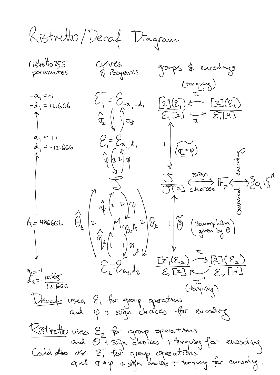
Conceptual Diagram
The following conceptual diagram relates Decaf and Ristretto. More details on its interpretation will be added in the future.
The right-hand column, groups & encodings, connects the byte strings produced by the encoding (middle, far right), to the quotient group constructed by Ristretto (bottom, far right), via all intermediate structures. (In practice, the encoding formulas pass directly from beginning to end; this is a conceptual diagram).
The center column, curves & isogenies, shows the relevant curves and their relationships.
The left-hand column, ristretto255 parameters, shows the concrete
parameter choices used for ristretto255.
Encoding in Affine Coordinates
We can write the Ristretto encoding/decoding procedure in affine coordinates, before describing optimized formulas to and from projective coordinates.
Encoding
On input \( (x,y) \in [2](\mathcal E)\), a representative for a coset in \( [2](\mathcal E) / \mathcal E[4] \):
-
Check if \( xy \) is negative or \( x = 0 \); if so, torque the point by setting \( (x,y) \gets (x,y) + Q_4 \), where \(Q_4\) is a \(4\)-torsion point.
-
Check if \(x\) is negative or \( y = -1 \); if so, set \( (x,y) \gets (x,y) + (0,-1) = (-x, -y) \).
-
Compute $$ s = +\sqrt {(-a) \frac {1 - y} {1 + y} }, $$ choosing the positive square root.
The output is then the (canonical) byte-encoding of \(s\).
If \(\mathcal E\) has cofactor \(4\), we skip the first step, since our input already represents a coset in \( [2](\mathcal E) / \mathcal E[2] \).
Interpreting the Encoding Procedure
How does this procedure correspond to the description involving \( \theta \)?
The first step lifts from \( \mathcal E / \mathcal E[4] \) to \(\mathcal E / \mathcal E[2]\). To understand steps 2 and 3, notice that the \(y\)-coordinate of \(\theta(s,t)\) is $$ y = \frac {1 + as^2}{1 - as^2}, $$ so that the \(s\)-coordinate of \(\theta^{-1}(x,y)\) has $$ s^2 = (-a)\frac {1-y}{1+y}. $$ Since $$ x = \frac 1 {\sqrt {ad - 1}} \frac {2s} {t}, $$ we also have $$ \frac s t = x \frac {\sqrt {ad-1}} 2, $$ so that the sign of \(s/t\) is determined by the sign of \(x\).
Recall that to choose a canonical representative of \( (s,t) + \mathcal J[2] \), it's sufficient to make two sign choices: the sign of \(s\) and the sign of \(s/t\). Step 2 determines the sign of \(s/t\), while step 3 computes \(s\) and determines its sign (by choosing the positive square root). Finally, the check that \(y \neq -1\) prevents division-by-zero when encoding the identity. If the inverse square root function returns \(0\), this check falls out of the optimized formulas for projective coordinates.
Decoding
On input s_bytes, decoding proceeds as follows:
-
Decode
s_bytesto \(s\); reject ifs_bytesis not the canonical encoding of \(s\). -
Check whether \(s\) is negative; if so, reject.
-
Compute $$ y \gets \frac {1 + as^2}{1 - as^2}. $$
-
Compute $$ x \gets +\sqrt{ \frac{4s^2} {ad(1+as^2)^2 - (1-as^2)^2}}, $$ choosing the positive square root, or reject if the square root does not exist.
-
Check whether \(xy\) is negative or \(y = 0\); if so, reject.
Encoding in Extended Coordinates
The formulas on the previous page are given in affine coordinates, but the usual internal representation is extended twisted Edwards coordinates \( (X:Y:Z:T) \) with \( x = X/Z \), \(y = Y/Z\), \(xy = T/Z \).
This presents a complication for the cofactor-\(8\) case: selecting the distinguished representative of the coset requires the affine coordinates \( (x,y) \), and computing \( s \) requires an inverse square root. As inversions are expensive, we'd like to be able to do this whole computation with only one inverse square root, by batching together the inversion and the inverse square root.
It is not obvious how to do this, since we need the inverse square root of one of two values, depending on what the distinguished representative is, but the choice of representative depends on the affine coordinates. However, an ingenious trick (due to Mike Hamburg) allows recovering either of the inverse square roots we want.
Batching the Inversion and Inverse Square Root
Write \( (X_0 : Y_0 : Z_0 : T_0) \) for the coordinates of the initial representative, and write \( (X:Y:Z:T) \) for the coordinates of the distinguished representative of the coset.
Since \(y = Y/Z\), in extended coordinates the formula for \(s\) becomes $$ s = \sqrt{ (-a) \frac{ 1 - Y/Z}{1+Y/Z}} = \sqrt{\frac{Z - Y}{Z+Y}} \sqrt{-a} = \frac {Z - Y} {\sqrt{Z^2 - Y^2}} \sqrt{-a}, $$ so we need to compute \( 1 / \sqrt{Z^2 - Y^2} \).
The distinguished representative \( (X:Y:Z:T) \) is selected by the torquing procedure in step 1, which conditionally adds a \(4\)-torsion point \(Q_4\). As noted in the torquing section above, \( Q_4 = (\pm 1/\sqrt{a}, 0) \), so we obtain $$ (X : Y : Z : T ) = \begin{cases} (X_0 : Y_0 : Z_0 : T_0) \\ (\pm Y_0 / \sqrt{a} : \mp X_0 \sqrt{a} : Z_0 : -T_0) \end{cases} . $$ This means we want to compute either of $$ \frac {1} {\sqrt{Z^2 - Y^2}} = \begin{cases} 1 / \sqrt{Z_0^2 - Y_0^2} \\ 1 / \sqrt{Z_0^2 - aX_0^2} \end{cases} . $$ To relate these quantities, recall from the curve equation that $$ -dX^2Y^2 = Z^4 - aZ^2X^2 - Z^2Y^2, $$ so $$ (a-d)X^2Y^2 = Z^4 - aZ^2X^2 - Z^2Y^2 + aX^2Y^2. $$ Factoring the right-hand side gives $$ (a-d)X^2Y^2 = (Z^2 - Y^2)(Z^2 - aX^2), $$ which relates the two quantities we want to compute: $$ \frac 1 {Z^2 - aX^2} = \frac 1 {a - d} \frac {Z^2 - Y^2} {X^2 Y^2}, $$ so $$ \frac 1 {\sqrt{Z^2 - aX^2}} = \frac 1 {\sqrt{a - d}} \sqrt{ \frac {Z^2 - Y^2} {X^2 Y^2} }. $$
Explicit Encoding Formulas
Using this trick, we can write the encoding procedure explicitly:
- \(u_1 \gets (Z_0 + Y_0)(Z_0 - Y_0) \textcolor{gray}{= Z_0^2 - Y_0^2} \)
- \(u_2 \gets X_0 Y_0 \)
- \(I \gets \mathrm{invsqrt}(u_1 u_2^2) \textcolor{gray}{= 1/\sqrt{X_0^2 Y_0^2 (Z_0^2 - Y_0^2)}} \)
- \(D_1 \gets u_1 I \textcolor{gray}{= \sqrt{(Z_0^2 - Y_0^2)/(X_0^2 Y_0^2)} } \)
- \(D_2 \gets u_2 I \textcolor{gray}{= \pm \sqrt{1/(Z_0^2 - Y_0^2)} } \)
- \(Z_{inv} \gets D_1 D_2 T_0 \textcolor{gray}{= (u_1 u_2)/(u_1 u_2^2) T_0 = T_0 / X_0 Y_0 = 1/Z_0} \)
- If \( T_0 Z_{inv} \textcolor{gray}{= x_0 y_0 }\) is negative:
- \( (X, Y) \gets (Y_0 (\pm 1/\sqrt{a}), X_0 (\mp \sqrt{a})) \)
- \( D \gets D_1 / \sqrt{a-d} \textcolor{gray}{= 1/\sqrt{Z_0^2 - a X_0^2} = 1/\sqrt{Z^2 -Y^2} } \)
- Otherwise:
- \( (X, Y) \gets (X_0, Y_0) \)
- \( D \gets D_2 \textcolor{gray}{= \pm \sqrt{1/(Z_0^2 - Y_0^2)} = \pm 1/\sqrt{Z^2 - Y^2}} \)
- If \( X Z_{inv} \textcolor{gray}{= x} \) is negative, set \( Y \gets - Y\)
- Compute \( s \gets |\sqrt{-a} (Z - Y) D| \textcolor{gray}{= |\sqrt{-a} (Z - Y) / \sqrt{Z^2 - Y^2}| } \)
- Return the canonical byte encoding of \( s \).
The choice of \( Q_4 = (i, 0) \) when \( a = -1 \) is convenient since it simplifies 7.1 to \( (X,Y) \gets (iY_0, iX_0) \).
Explicit Decoding Formulas
As with encoding, we want to batch operations to use only a single inverse square root. However, the procedure is much simpler since there's no torquing.
On input s_bytes:
- Check that
s_bytesis the canonical byte-encoding of a field element \(s\), otherwise reject. - Decode
s_bytesto \(s\). - Check that \( s \) is nonnegative, otherwise reject.
- \( u_1 \gets 1 + as^2 \)
- \( u_2 \gets 1 - as^2 \)
- \( v \gets (ad)u_1^2 - u_2^2 \textcolor{gray}{= ad(1+as^2)^2 - (1-as^2)^2} \)
- \( I \gets \mathrm{invsqrt}( v u_2^2 ) \textcolor{gray}{= 1/\sqrt{v u_2^2} } \)
- \( D_x \gets Iu_2 \textcolor{gray}{= 1/\sqrt{v} } \)
- \( D_y \gets ID_x v \textcolor{gray}{= I^2 u_2 v = (v u_2) / (v u_2^2) = 1/u_2 } \)
- \( x \gets |2sD_x| \textcolor{gray}{= +\sqrt{ 4s^2 / (ad(1+as^2)^2 - (1-as^2)^2 )}}\)
- \( y \gets u_1 D_y \textcolor{gray}{= (1+as^2)/(1-as^2) } \)
- \( t \gets xy \)
- Check that \(t \) is nonnegative and that \( y \neq 0 \), otherwise reject.
- Return \( P = (x: y: 1: t) \)
TODO
Add explicit formulas for the cofactor 4 case.
Equality Testing
Testing equality of two Ristretto points means testing whether they are equal in the quotient group, i.e., whether they lie in the same coset of \(\mathcal E[4] \) (for the cofactor-\(8\) case) or \(\mathcal E[2] \) (for the cofactor-\(4\) case).
Equality testing of points on the Edwards curve requires comparing to affine coordinates, which requires an expensive inversion. However, testing whether two points lie in the same coset can be done in projective coordinates, making it actually easier than equality testing in the original non-quotient group.
The Decaf paper proves that in the cofactor-\(4\) case, to test equality of \(P_1 = (X_1:Y_1:Z_1:T_1)\) and \(P_2 = (X_2:Y_2:Z_2:T_2)\) it's sufficient to test whether \[ X_1 Y_2 = Y_1 X_2. \]
In the cofactor-\(8\) case, we need to test equality not modulo \(\mathcal E[2]\) but modulo \(\mathcal E[4]\). This means we need to check whether either \( P_1 \equiv P_2 \pmod {\mathcal E[2]} \) or \( P_1 + Q_4 \equiv P_2 \pmod {\mathcal E[2]} \), where \(Q_4\) is a \(4\)-torsion point.
Write \(P_1 + Q_4 = (X_1' : Y_1' : Z_1' : T_1')\). In affine coordinates, \(P + Q_4 = (y/\sqrt a, -x\sqrt a)\), so that \(X_1' = Y_1 / \sqrt a\), \(Y_1' = -X_1 \sqrt a\). The equation \[ X_1' Y_2 = Y_1' X_2 \] then becomes \[ Y_1 Y_2 / \sqrt a = - \sqrt a X_1 X_2 \] or equivalently \[ Y_1 Y_2 = - a X_1 X_2. \]
So, to check equality modulo \(\mathcal E[4]\), it's sufficient to check whether \[ X_1 Y_2 = Y_1 X_2 \quad \mathrm{or} \quad Y_1 Y_2 = -a X_1 X_2. \]
Elligator
The Decaf paper explains how to formulate a map from field elements to points suitable for hashing to group elements. Rather than mapping directly to the Edwards or Montgomery model, Decaf suggests using Elligator 2 to the Jacobi quartic \(\mathcal J\), then applying an isogeny to obtain a point on whichever curve is used for implementing group operations. This allows implementations using different curves internally to have compatible Elligator maps.
This method also applies to Ristretto, with a suitable change of variables.
Elligator for Decaf
The Decaf paper constructs the Elligator map as follows, using the Decaf parameters \(a_1, d_1\). First, fix a parameter \(n \in \mathbb F \) which is nonsquare. Then, on input \(r_0 \in \mathbb F\), compute \( r \gets n r_0^2 \). Since \( n \) is nonsquare, \(r\) is nonsquare unless \(r_0 = 0\), in which case \(r = 0\).
The output of the Elligator map is either \[ (s,t) = \left( + \sqrt{ \frac{ (r+1)(a_1 - 2d_1) }{ (d_1 r + a_1 - d_1) (d_1 r - a_1 r - d_1) } } , \frac{ -(r-1)(a_1 - 2d_1)^2 }{ (d_1 r + a_1 - d_1) (d_1 r - a_1 r - d_1) } - 1 \right) \] or \[ (s,t) = \left( - \sqrt{ \frac{ r(r+1)(a_1 - 2d_1) }{ (d_1 r + a_1 - d_1) (d_1 r - a_1 r - d_1) } } , \frac{ r(r-1)(a_1 - 2d_1)^2 }{ (d_1 r + a_1 - d_1) (d_1 r - a_1 r - d_1) } - 1 \right) \] depending on which square root exists, preferring the second case when \(r = 0\) and both are square.
Changing variables to Ristretto parameters
We can rewrite this in terms of the Ristretto parameters \(a_2, d_2\) using the identities \(a_1 = -a_2\), \(d_1 = a_2d_2 / (a_2 - d_2)\). The denominator is \[ \begin{aligned} D &= (d_1 r + a_1 - d_1) (d_1 r - a_1 r - d_1) \\ &= \left( \frac {a_2 d_2}{ a_2 - d_2} r - a_2 - \frac {a_2 d_2}{ a_2 - d_2} \right) \left( \frac {a_2 d_2}{ a_2 - d_2} r + a_2r - \frac {a_2 d_2}{ a_2 - d_2} \right) \\ &= \frac { \left( a_2 d_2 r - a_2(a_2 - d_2) - a_2 d_2 \right) \left( a_2 d_2 r + a_2(a_2 -d_2) r - a_2 d_2 \right) } {(a_2 - d_2)^2} \\ &= \frac { \left( a_2 d_2 r - 1 \right) \left( r - a_2 d_2 \right) } {(a_2 - d_2)^2} . \\ \end{aligned} \] Since \(a_2^2 = 1\), this is \[ \begin{aligned} D &= \frac { a_2^2 \left( a_2 d_2 r - 1 \right) \left( r - a_2 d_2 \right) } {(a_2 - d_2)^2} \\ &= \frac { \left( a_2^2 d_2 r - a_2 \right) \left( a_2 r - a_2^2 d_2 \right) } {(a_2 - d_2)^2} \\ &= \frac { \left( d_2 r - a_2 \right) \left( a_2 r - d_2 \right) } {(a_2 - d_2)^2} , \\ \end{aligned} \] so that \[ 1/D = \frac {(a_2 - d_2)^2} { \left( d_2 r - a_2 \right) \left( a_2 r - d_2 \right) } . \] The numerators of the terms in the Elligator map are \[ \begin{aligned} (r+1)(a_1 - 2d_1) &\qquad & -(r+1)(a_1 - 2d_1)^2 \\ r(r+1)(a_1 - 2d_1) & \qquad & r(r+1)(a_1 - 2d_1)^2; \\ \end{aligned} \] since \[ a_1 - 2d_1 = - a_2 \left( \frac{a_2 + d_2}{a_2 - d_2} \right)^2, \] these become \[ \begin{aligned} -a_2 (r+1) \left( \frac{a_2 + d_2}{a_2 - d_2} \right) &\qquad & +a_2 (r-1) \left( \frac{a_2 + d_2}{a_2 - d_2} \right)^2 \\ -a_2 r (r+1) \left( \frac{a_2 + d_2}{a_2 - d_2} \right) & \qquad & -a_2 r (r-1) \left( \frac{a_2 + d_2}{a_2 - d_2} \right)^2. \\ \end{aligned} \] Multiplying the numerators by the denominator \(1/D\) gives \[ \begin{aligned} \frac { -a_2 (r+1) (a_2 + d_2)(a_2 - d_2) }{ (d_2 r - a_2)(a_2r-d_2) } &\qquad & \frac { +a_2 (r-1) (a_2 + d_2)^2 }{ (d_2 r - a_2)(a_2r-d_2) } \\ \frac { -a_2 r (r+1) (a_2 + d_2)(a_2 - d_2) }{ (d_2 r - a_2)(a_2r-d_2) } & \qquad & \frac { -a_2 r (r-1) (a_2 + d_2)^2 }{ (d_2 r - a_2)(a_2r-d_2) } \\ \end{aligned} \]
Elligator for Ristretto
The Elligator map, written in terms of the Ristretto parameters, is therefore given by \[ (s,t) = \left( + \sqrt{ \frac{ a_2(r+1)(a_2 + d_2)(d_2 - a_2) }{ (d_2 r - a_2)(a_2 r - d_2) } } , \frac{ +a_2(r-1)(a_2 + d_2)^2 }{ (d_2 r - a_2)(a_2 r - d_2) } - 1 \right) \] or \[ (s,t) = \left( - \sqrt{ \frac{ a_2r(r+1)(a_2 + d_2)(d_2 - a_2) }{ (d_2 r - a_2)(a_2 r - d_2) } } , \frac{ -a_2r(r-1)(a_2 + d_2)^2 }{ (d_2 r - a_2)(a_2 r - d_2) } - 1 \right) \] depending on which square root exists, preferring the second when \(r = 0\) and both are square.
Elligator in Extended Coordinates
As noted on the previous page, the Elligator map to the Jacobi
quartic, written in terms of the Ristretto parameters, is given by
\[
(s,t) =
\left(
+ \sqrt{
\frac{
a_2(r+1)(a_2 + d_2)(d_2 - a_2)
}{
(d_2 r - a_2)(a_2 r - d_2)
}
}
,
\frac{
+a_2(r-1)(a_2 + d_2)^2
}{
(d_2 r - a_2)(a_2 r - d_2)
}
- 1
\right)
\]
or
\[
(s,t) =
\left(
- \sqrt{
\frac{
a_2r(r+1)(a_2 + d_2)(d_2 - a_2)
}{
(d_2 r - a_2)(a_2 r - d_2)
}
}
,
\frac{
-a_2r(r-1)(a_2 + d_2)^2
}{
(d_2 r - a_2)(a_2 r - d_2)
}
- 1
\right)
\]
depending on which square root exists, preferring the second when \(r
= 0\) and both are square. (When using the ristretto255
parameters, the first is nonsquare when \(r = 0\)
and there is no ambiguity).
Applying the isogeny \(\theta\) to \(s,t\) gives a point on \(\mathcal E_2\). When the denominator is zero, the Elligator result should be a 2-torsion point, but as noted in the Decaf paper it does not matter which one, since we quotient out by \(2\)-torsion anyways.
Elligator for ristretto255 in extended coordinates
This can be implemented for ristretto255 with a single square root
computation, using the sqrt_ratio_i function described in the
explicit formulas section. To make this
work, ristretto255 chooses \(n = i = +\sqrt{-1}\) as the quadratic
nonresidue.
Write the numerator and denominator as \[ \begin{aligned} N_s &= a(r+1)(a + d)(d - a) \\ D &= (d r - a)(a r - d). \end{aligned} \] The value of \(s\) is then either \(+\sqrt{N_s/D}\) or \(-\sqrt{rN_s/D}\). Since \(r = ir_0^2\), we have \[ -\sqrt{\frac {rN_s} D} = -\sqrt{\frac {ir_0^2N_s} D} = -\left| r_0 \sqrt{i \frac {N_s} D} \right|. \]
Because we want to apply \(\theta\) to \((s,t)\), we can work projectively and write \(t = N_t/D\). Then \[ N_t = c(r-1)(a+d)^2 - D, \] where \(c = a\) in the first case where \(N_s/D\) is square and \(c = -ar\) in the second case where \(rN_s/D\) is square.
Applying \(\theta\) gives \[ (x,y) = \left( \frac { 2s } { t } \frac 1 { \sqrt{ad-1} } , \quad \frac { 1 +a s^2 } { 1 - as^2 } \right) = \left( \frac { 2s D } { N_t \sqrt{ad-1} } , \quad \frac { 1 + as^2 } { 1 - a s^2 } \right). \] In extended coordinates, this becomes \[ \begin{aligned} X &= (2sD)(1-as^2) \\ Y &= (1+as^2)(N_t \sqrt{ad-1})\\ Z &= (N_t \sqrt{ad-1})(1-as^2)\\ T &= (2sD)(1+as^2). \end{aligned} \]
In summary, we can compute the Elligator map directly to extended coordinates as follows.
- \(r \gets ir_0^2\).
- \(N_s \gets (r+1)(1-d^2) \textcolor{gray}{= a(r+1)(a+d)(a-d)} \).
- \(c \gets -1\).
- \(D \gets (c - dr)(r+d) \textcolor{gray}{= (dr -a)(ar-d)} \).
Ns_D_is_sq, \(s \gets \)sqrt_ratio_i(N_s, D).- \(s' \gets -|s r_0|\).
- \(s \gets s' \) if not
Ns_D_is_sq. - \(c \gets r \) if not
Ns_D_is_sq. - \(N_t \gets c(r-1)(d-1)^2 - D\).
- \(W_0 \gets 2sD \).
- \(W_1 \gets N_t\sqrt{ad-1} \).
- \(W_2 \gets 1 - s^2 \textcolor{gray}{= 1 +as^2} \).
- \(W_3 \gets 1 + s^2 \textcolor{gray}{= 1 -as^2} \).
- Return \( (W_0 W_3 : W_2 W_1 : W_1 W_3 : W_0 W_2) \).
When \(D = 0\), we need to obtain a \(2\)-torsion point, but since
sqrt_ratio_i returns (0, 0), the resulting Edwards point will be
the identity \((0,1)\), so the exceptional case does not need to be
handled specially.
Batched Double-and-Encode
The encoding is not batchable, since it requires an inverse square root. However, since \( \theta \circ \hat \theta = [2] P \), it's possible to compute the encoding of \( [2]P \) by using \( \hat \theta \) instead of \( \theta^{-1} \). Since \( \hat \theta \) only requires inversions, given \( P_1, \ldots, P_n \), it's possible to compute the encodings of \( [2]P_1, \ldots, [2]P_n \) in a batch.
XXX write up details
Explicit Formulas
As mentioned in the What is Ristretto chapter, Ristretto defines a new point type, together with formulas for encoding, decoding, equality checking, and hash-to-point operations.
This chapter contains explicit formulas for these operations, aimed at implementors.
A note on type safety
Ristretto points are represented by curve points, but they are not curve points. Not every curve point is a representative of a Ristretto point. The Ristretto group is not a subgroup of the curve, and the Ristretto group is logically distinct from the group of curve points.
For these reasons, Ristretto points should have a different type than curve points, and it should be a type error to mix them. In particular, it's dangerous and unsafe to implement the Ristretto functions as operating on arbitrary curve points, rather than only on the representatives contained in a distinct Ristretto point type.
Implementation
Implementing Ristretto using an existing Edwards curve implementation requires the following:
- A distinct type for Ristretto points which forwards curve operations on points to their corresponding canonical representative in the Ristretto group (as mentioned in the previous section);
- A function for decoding (so that only the canonical encoding of a coset is accepted);
- A function for encoding (so that two representatives of the same coset are encoded as identical bitstrings);
- A function for equality checking (so that two representatives of the same coset are considered equal);
- A function for hashing to the Ristretto group.
Implementation of these functions requires an inverse square root
function. This is often inlined into a point decompression function,
so we also give formulas for implementing an inverse square root for
ristretto255.
Extracting an Inverse Square Root
Implementing Ristretto requires computing (inverse) square roots. Ed25519 implementations compute square roots as part of the Ed25519 decompression functionality, but this is often inlined into the decompression formulas.
This page explains how to extract an inverse square root function
suitable for use with ristretto255 from an implementation of Ed25519.
Computing \(\sqrt{u/v}\) or \(\sqrt{iu/v}\) simultaneously
Let \(p = 2^{255} -19\). On input field elements \(u, v\), set \[ r = (uv^3)(uv^7)^{(p-5)/8}. \]
There are four possibilities when \(u,v\) are nonzero:
- If \(vr^2 = u\), then \( s \gets r \) is a square root of \(u/v\).
- If \(vr^2 = -u\), then \( s \gets ir \) is a square root of \(u/v\).
- If \(vr^2 = iu\), then \( s \gets r \) is a square root of \(iu/v\).
- If \(vr^2 = -iu\), then \( s \gets ir \) is a square root of \(iu/v\).
When \(u = 0\), \(r = 0\) and the first condition \(vr^2 = u\) is satisfied. When \(v = 0\) and \(u \neq 0\), \(r = 0\) and none of the conditions are satisfied. This allows computing the nonnegative square root of either \( \sqrt{u/v} \) or \(\sqrt{iu/v}\) as follows:
- \(r \gets (uv^3)(uv^7)^{(p-5)/8}\).
- \(c \gets vr^2\).
correct_sign_sqrt\(\gets (c = u)\).flipped_sign_sqrt\(\gets (c = -u)\).flipped_sign_sqrt_i\(\gets (c = -iu)\).- \( r \gets ir \) if
flipped_sign_sqrt | flipped_sign_sqrt_i. - \( r \gets -r \) if \(r\) is negative.
- Return
(correct_sign_sqrt | flipped_sign_sqrt, r).
The first part of the return value signals whether \(u/v\) was square, and the second part contains a square root. Specifically, it returns
( true, +sqrt(u/v))if \(v\) is nonzero and \(u/v\) is square;( true, zero)if \(u\) is zero;(false, zero)if \(v\) is zero and \(u\) is nonzero;(false, +sqrt(i*u/v))if \(u/v\) is nonsquare (so \(iu/v\) is square).
The computation of \(x^{(p-5)/8}\) is already required for Ed25519
decoding, so an Ed25519 implementation can obtain a sqrt_ratio_i
function by refactoring the computation of \(r\) out of the decoding
function and using sqrt_ratio_i to perform decoding.
If the equality checks in (3), (4), (5) are implemented in constant-time and the conditional assignments in (6), (7) are also implemented in constant-time, then the entire computation can be done in constant time.
Decoding to Extended Coordinates
To decode a byte-string s_bytes representing a compressed Ristretto
point into extended coordinates, an implementation proceeds as
follows.
- Check that
s_bytesis the canonical encoding of a field element, or else abort. - Decode
s_bytes, a byte-string, into \(s\), a field element. - Check that \(s\) is non-negative, or else abort.
- \(u_1 \gets 1 + a s^{2} \).
- \(u_2 \gets 1 - a s^{2} \).
- \(v \gets adu_1^2 - u_2^2 \).
- \(I \gets \mathrm{invsqrt}( v u_2^{2} ) \), or abort if the square root does not exist.
- \(D_x \gets I u_2 \).
- \(D_y \gets I D_x v \).
- \(x \gets |2 s D_x| \), i.e., compute \(2sD_x\) and negate it if it is negative.
- Compute \(y \gets u_1 D_y \).
- Compute \(t \gets x y \).
- If \( t \) is negative or \( y = 0 \), abort. Otherwise, return the Ristretto point represented by \(( x: y: 1: t \)).
Since \( a = \pm 1 \), implementations can replace multiplications by \(a\) with sign changes, as appropriate.
If the implementation's field element encoding function produces
canonical outputs, one way to check that s_bytes is a canonical
encoding (in step 1) is to decode s_bytes into \(s\), then
re-encode \(s\) into s_bytes_check, and ensure that s_bytes == s_bytes_check.
The ristretto255 test vectors include checks for non-canonical decoding.
Encoding from Extended Coordinates
To encode a Ristretto point represented by the point \((X:Y:Z:T)\) in extended coordinates, an implementation proceeds as follows.
- \(u_1 \gets (Z_0 + Y_0)(Z_0 - Y_0) \).
- \(u_2 \gets X_0 Y_0 \).
- \(I \gets \mathrm{invsqrt}(u_1 u_2^2) \).
- \(D_1 \gets u_1 I \).
- \(D_2 \gets u_2 I \).
- \(Z_{inv} \gets D_1 D_2 T_0 \).
- If \( T_0 Z_{inv} \) is negative:
- \( (X, Y) \gets (Y_0 (\pm 1/\sqrt{a}), X_0 (\mp \sqrt{a})) \).
- \( D \gets D_1 / \sqrt{a-d} \).
- Otherwise:
- \( (X, Y) \gets (X_0, Y_0) \).
- \( D \gets D_2 \).
- If \( X Z_{inv} \) is negative, set \( Y \gets - Y\).
- Compute \( s \gets |\sqrt{-a} (Z - Y) D| \), i.e., compute \(\sqrt{-a} (Z - Y) D\) and negate it if it is negative.
- Return the canonical byte encoding of \( s \).
Since \( a = \pm 1 \), implementations can replace multiplications by \(a\) with sign changes, as appropriate.
When \(a = -1\), (10) becomes \(s \gets |(Z-Y)D|\), and choosing \( Q_4 = (i, 0) \) is convenient since it simplifies (7.1) to \( (X,Y) \gets (iY_0, iX_0) \).
The inverse square root in step 3 always exists when \((X:Y:Z:T)\) is a valid representative.
Testing Equality
To test equality of two Edwards points \(P_1 = (X_1:Y_1:Z_1:T_1)\) and \(P_2 = (X_2:Y_2:Z_2:T_2)\) which represent Ristretto points, it's sufficient to check whether \[ X_1 Y_2 = Y_1 X_2 \quad \mathrm{or} \quad Y_1 Y_2 = -a X_1 X_2. \]
Note that when \(a = -1\), this simplifies to \[ X_1 Y_2 = Y_1 X_2 \quad \mathrm{or} \quad Y_1 Y_2 = X_1 X_2. \]
Unlike testing equality on the Edwards curve, this does not require an inversion and can be done in projective coordinates.
Hash-to-Group with Elligator
The hash-to-group operation applies Elligator twice and adds the results.
Hash-to-ristretto255
Given bytes, 64 bytes of hash output, construct field elements \(r_0, r_1\) as
- \(r_0\) is the low 255 bits of
bytes[ 0..32], taken mod \(p\). - \(r_1\) is the low 255 bits of
bytes[32..64], taken mod \(p\).
Apply the Elligator map below to the inputs \(r_0, r_1\) to obtain points \(P_1, P_2\), and return \(P_1 + P_2\).
- \(r \gets ir_0^2\).
- \(N_s \gets (r+1)(1-d^2) \textcolor{gray}{= a(r+1)(a+d)(a-d)} \).
- \(c \gets -1\).
- \(D \gets (c - dr)(r+d) \textcolor{gray}{= (dr -a)(ar-d)} \).
Ns_D_is_sq, \(s \gets \)sqrt_ratio_i(N_s, D).- \(s' \gets -|s r_0|\).
- \(s \gets s' \) if not
Ns_D_is_sq. - \(c \gets r \) if not
Ns_D_is_sq. - \(N_t \gets c(r-1)(d-1)^2 - D\).
- \(W_0 \gets 2sD \).
- \(W_1 \gets N_t\sqrt{ad-1} \).
- \(W_2 \gets 1 - s^2 \textcolor{gray}{= 1 +as^2} \).
- \(W_3 \gets 1 + s^2 \textcolor{gray}{= 1 -as^2} \).
- Return \( (W_0 W_3 : W_2 W_1 : W_1 W_3 : W_0 W_2) \).
Test vectors for ristretto255
ristretto255 encodes group elements using 255 bits and provides a
prime-order group of size 2^252. It can be implemented using
Curve25519.
For ristretto255, the parameters are
\[
\begin{aligned}
p &= 2^{255}-19 \\
a_2 = a &= -1 \\
d_2 = d &= -121665/121666.
\end{aligned}
\]
Field elements are considered negative when their low bit is set, as in Ed25519.
The Elligator map uses \(n = +\sqrt{-1}\) as the quadratic nonresidue.
// The test vectors below also have code to test them against the
// curve25519_dalek implementation.
//
// These tests are run in CI against the curve25519-dalek implementation.

extern crate sha2;
extern crate hex;
extern crate curve25519_dalek;

# fn main() {
// The following are the byte encodings of small multiples
//     [0]B, [1]B, ..., [15]B
// of the basepoint, represented as hex strings.

let encodings_of_small_multiples = [
    // This is the identity point
    "0000000000000000000000000000000000000000000000000000000000000000",
    // This is the basepoint
    "e2f2ae0a6abc4e71a884a961c500515f58e30b6aa582dd8db6a65945e08d2d76",
    // These are small multiples of the basepoint
    "6a493210f7499cd17fecb510ae0cea23a110e8d5b901f8acadd3095c73a3b919",
    "94741f5d5d52755ece4f23f044ee27d5d1ea1e2bd196b462166b16152a9d0259",
    "da80862773358b466ffadfe0b3293ab3d9fd53c5ea6c955358f568322daf6a57",
    "e882b131016b52c1d3337080187cf768423efccbb517bb495ab812c4160ff44e",
    "f64746d3c92b13050ed8d80236a7f0007c3b3f962f5ba793d19a601ebb1df403",
    "44f53520926ec81fbd5a387845beb7df85a96a24ece18738bdcfa6a7822a176d",
    "903293d8f2287ebe10e2374dc1a53e0bc887e592699f02d077d5263cdd55601c",
    "02622ace8f7303a31cafc63f8fc48fdc16e1c8c8d234b2f0d6685282a9076031",
    "20706fd788b2720a1ed2a5dad4952b01f413bcf0e7564de8cdc816689e2db95f",
    "bce83f8ba5dd2fa572864c24ba1810f9522bc6004afe95877ac73241cafdab42",
    "e4549ee16b9aa03099ca208c67adafcafa4c3f3e4e5303de6026e3ca8ff84460",
    "aa52e000df2e16f55fb1032fc33bc42742dad6bd5a8fc0be0167436c5948501f",
    "46376b80f409b29dc2b5f6f0c52591990896e5716f41477cd30085ab7f10301e",
    "e0c418f7c8d9c4cdd7395b93ea124f3ad99021bb681dfc3302a9d99a2e53e64e",
];

// Test the encodings of small multiples

use curve25519_dalek::constants;
use curve25519_dalek::traits::Identity;
use curve25519_dalek::ristretto::RistrettoPoint;

let B = &constants::RISTRETTO_BASEPOINT_POINT;
let mut P = RistrettoPoint::identity();
for i in 0..16 {
    assert_eq!(
        hex::encode(P.compress().as_bytes()),
        encodings_of_small_multiples[i],
    );
    P = P + B;
}

// The following are invalid encodings, which should all be rejected.
// These are designed to test each of the checks during decoding.

let bad_encodings = [
    // These are all bad because they're non-canonical field encodings.
    "00ffffffffffffffffffffffffffffffffffffffffffffffffffffffffffffff",
    "ffffffffffffffffffffffffffffffffffffffffffffffffffffffffffffff7f",
    "f3ffffffffffffffffffffffffffffffffffffffffffffffffffffffffffff7f",
    "edffffffffffffffffffffffffffffffffffffffffffffffffffffffffffff7f",
    // These are all bad because they're negative field elements.
    "0100000000000000000000000000000000000000000000000000000000000000",
    "01ffffffffffffffffffffffffffffffffffffffffffffffffffffffffffff7f",
    "ed57ffd8c914fb201471d1c3d245ce3c746fcbe63a3679d51b6a516ebebe0e20",
    "c34c4e1826e5d403b78e246e88aa051c36ccf0aafebffe137d148a2bf9104562",
    "c940e5a4404157cfb1628b108db051a8d439e1a421394ec4ebccb9ec92a8ac78",
    "47cfc5497c53dc8e61c91d17fd626ffb1c49e2bca94eed052281b510b1117a24",
    "f1c6165d33367351b0da8f6e4511010c68174a03b6581212c71c0e1d026c3c72",
    "87260f7a2f12495118360f02c26a470f450dadf34a413d21042b43b9d93e1309",
    // These are all bad because they give a nonsquare x^2.
    "26948d35ca62e643e26a83177332e6b6afeb9d08e4268b650f1f5bbd8d81d371",
    "4eac077a713c57b4f4397629a4145982c661f48044dd3f96427d40b147d9742f",
    "de6a7b00deadc788eb6b6c8d20c0ae96c2f2019078fa604fee5b87d6e989ad7b",
    "bcab477be20861e01e4a0e295284146a510150d9817763caf1a6f4b422d67042",
    "2a292df7e32cababbd9de088d1d1abec9fc0440f637ed2fba145094dc14bea08",
    "f4a9e534fc0d216c44b218fa0c42d99635a0127ee2e53c712f70609649fdff22",
    "8268436f8c4126196cf64b3c7ddbda90746a378625f9813dd9b8457077256731",
    "2810e5cbc2cc4d4eece54f61c6f69758e289aa7ab440b3cbeaa21995c2f4232b",
    // These are all bad because they give a negative xy value.
    "3eb858e78f5a7254d8c9731174a94f76755fd3941c0ac93735c07ba14579630e",
    "a45fdc55c76448c049a1ab33f17023edfb2be3581e9c7aade8a6125215e04220",
    "d483fe813c6ba647ebbfd3ec41adca1c6130c2beeee9d9bf065c8d151c5f396e",
    "8a2e1d30050198c65a54483123960ccc38aef6848e1ec8f5f780e8523769ba32",
    "32888462f8b486c68ad7dd9610be5192bbeaf3b443951ac1a8118419d9fa097b",
    "227142501b9d4355ccba290404bde41575b037693cef1f438c47f8fbf35d1165",
    "5c37cc491da847cfeb9281d407efc41e15144c876e0170b499a96a22ed31e01e",
    "445425117cb8c90edcbc7c1cc0e74f747f2c1efa5630a967c64f287792a48a4b",
    // This is s = -1, which causes y = 0.
    "ecffffffffffffffffffffffffffffffffffffffffffffffffffffffffffff7f",
];

// Test that all of the bad encodings are rejected

use curve25519_dalek::ristretto::CompressedRistretto;

let mut bad_bytes = [0u8; 32];
for bad_encoding in &bad_encodings {
    bad_bytes.copy_from_slice(&hex::decode(bad_encoding).unwrap());
    assert!(CompressedRistretto(bad_bytes).decompress().is_none());
}

// The following are a list of UTF-8 encoded strings, and the byte
// encodings of performing hash-to-point with SHA-512.

let labels = [
    "Ristretto is traditionally a short shot of espresso coffee",
    "made with the normal amount of ground coffee but extracted with",
    "about half the amount of water in the same amount of time",
    "by using a finer grind.",
    "This produces a concentrated shot of coffee per volume.",
    "Just pulling a normal shot short will produce a weaker shot",
    "and is not a Ristretto as some believe.",
];

let encoded_hash_to_points = [
    "3066f82a1a747d45120d1740f14358531a8f04bbffe6a819f86dfe50f44a0a46",
    "f26e5b6f7d362d2d2a94c5d0e7602cb4773c95a2e5c31a64f133189fa76ed61b",
    "006ccd2a9e6867e6a2c5cea83d3302cc9de128dd2a9a57dd8ee7b9d7ffe02826",
    "f8f0c87cf237953c5890aec3998169005dae3eca1fbb04548c635953c817f92a",
    "ae81e7dedf20a497e10c304a765c1767a42d6e06029758d2d7e8ef7cc4c41179",
    "e2705652ff9f5e44d3e841bf1c251cf7dddb77d140870d1ab2ed64f1a9ce8628",
    "80bd07262511cdde4863f8a7434cef696750681cb9510eea557088f76d9e5065",
];

// Test the encodings above.

use sha2::{Sha512, Digest};

for i in 0..7 {
    let point = RistrettoPoint::hash_from_bytes::<Sha512>(labels[i].as_bytes());
    assert_eq!(
        hex::encode(point.compress().as_bytes()),
        encoded_hash_to_points[i],
    );
}
# }
ristretto255 Implementations
An internet-draft for ristretto255 is now available, written by Henry de Valence, Jack Grigg, George Tankersley, Filippo Valsorda, and Isis Lovecruft.
- Rust:
curve25519-dalek, by Isis Lovecruft and Henry de Valence; - Go:
ristretto255, by George Tankersley, Filippo Valsorda, and Henry de Valence; - C:
libsodium, by Frank Denis. - AssemblyScript:
wasm-crypto, by Frank Denis. - Javascript with Typescript:
noble-ed25519, by Paul Miller - Javascript:
ristretto255-js, by Valeria Nikolaenko and Kevin Lewi. - Zig: the
zigprogramming language includes ristretto255 in its standard library, implemented by Frank Denis.